Exercises

Variant calling

Variant Calling Tutorial

This tutorial will provide you with the practical skills needed to analyze next-generation sequencing data in a clinical and research context. Upon completion of this session, you will be able to:

Interpret sequencing evidence: master the use of Integrative Genomics Viewer (IGV) to visually inspect and validate genomic features, variant calls, and alignment artifacts.
Run a somatic call pipeline: apply a bioinformatics workflow based on best practices to accurately identify somatic variants from a matched pair of tumor and normal samples.
Predict functional impact: use tools such as the Variant Effect Predictor (VEP) to annotate variants and predict their biological consequences, from amino acid changes to effects on gene expression.
Prioritize actionable variants: develop a strategic approach to filter and prioritize mutations with the highest probability of being oncogenic drivers or therapeutic targets in a cancer genome.

As we proceed, code snippets will be provided to help you build the system step-by-step.

Attribution: This tutorial is inspired by the Precision medicine course, from the Griffith lab and Cancer variant analysis from SIB.

Tutorial Outline

Setup: Tools of the trade
IGV Tutorial: A Guide to Visualizing NGS Data
Data Quality: The First Step to Confident Calls
Variant Calling: The Art of Finding Genetic Changes
Variant Annotation and Filtering: Turning Variants into Insights

1. Setup

Tools of the trade

Setup: Tools of the trade

To perform the exercises, you need the following tools installed on your machine.

IGV
bcftools
GATK4
MultiQC
samtools
VEP

Alternatively, you can use the Singularity images available on GIT (you need Singularity).

Running IGV (Integrative Genomics Viewer) 💻

IGV is available as a powerful **Desktop Application** (Java-based) and a convenient **Web App** (JavaScript-based).

Option 1: IGV Web App (Recommended for Quick Access) ✅

If you don't already have the desktop version installed, the **Web App** is the fastest way to start viewing your data.


							# Go to the official Web App URL
							https://igv.org/app/

**No Installation** required—it runs entirely in your modern web browser.
Load files directly from your **local machine** or a **public URL** (e.g., BAM, VCF, BigWig).
No data is uploaded; the viewer runs as a secure, client-side application.

Option 2: IGV Desktop Application (For Full Power) 🚀

The desktop version provides a more robust and flexible experience, particularly for very large or complex datasets.

**Requires Java** and a local download (Windows, Mac, or Linux).
Allows you to allocate more **RAM** (memory) for extremely large-scale data files.
Provides access to **advanced tools** like IGVtools for local data manipulation.

Use the desktop version if you run into performance issues with the Web App or need advanced features.

Installing bcftools 🛠️

We recommend using a package manager like Conda/Mamba for simple, isolated installations.

Method 1: Conda/Mamba (Recommended)


							mamba create -n bcftools_env bcftools
							conda activate bcftools_env
							bcftools --version

Mamba is often faster than Conda.
The environment name (`bcftools_env`) is arbitrary.
This method handles dependencies automatically.

Method 2: From Source (Advanced)

Requires `git`, `make`, and `gcc` (or similar compiler).


							git clone --branch=develop https://github.com/samtools/bcftools.git
							cd bcftools
							make
							sudo make install

Remind: users that "make install" might require specifying an install path with PREFIX.

Verification

Run the help command to ensure it's installed correctly:


						bcftools

The output should display the usage summary.

Installing GATK4 (Genome Analysis Toolkit)

GATK is a Java-based tool, but **GATK4** has complex Python/R dependencies for tools like CNV and CNNScoreVariants.

Recommendation: Use a container or Conda/Mamba to manage dependencies.

Method 1: Conda / Mamba (Recommended for Local Use)

This is the most common way to get an isolated environment and automatically handle all dependencies.


						# 1. Create a Conda/Mamba environment
						mamba create -n gatk4_env gatk4 -c bioconda -c conda-forge
						# 2. Activate the environment
						conda activate gatk4_env
						# 3. Test the installation
						gatk --version

GATK4 requires **Java 1.8 (Java 8)** or newer, which Mamba installs automatically.

Method 2: Docker / Singularity (Best for HPC)

The Broad Institute provides official containers with everything pre-configured.


						# Docker command to pull the official image
						docker pull broadinstitute/gatk:latest

						# Docker command to run a simple tool
						docker run --rm broadinstitute/gatk:latest gatk --list

						# For Singularity (as mentioned in your context)
						singularity pull docker://broadinstitute/gatk:latest
						# Then run:
						singularity run gatk_latest.sif gatk --version

Using containers ensures **100% reproducibility** across different machines.

Method 3: Download Binaries (Requires Java & PATH Setup)

Download the ZIP archive from the official Broad Institute GitHub releases page.


							# 1. Download and unzip the package
							wget https://github.com/broadinstitute/gatk/releases/download/[VERSION]/gatk-[VERSION].zip
							unzip gatk-[VERSION].zip

							# 2. Add the wrapper script to your PATH
							export PATH="/path/to/gatk-package/:\$PATH"

You must have Java 8+ installed separately, and this method requires careful setup of Python/R dependencies for some tools.

Installing MultiQC 📊

MultiQC aggregates results from multiple bioinformatics tools (FastQC, Samtools, etc.) into a single, interactive report.

It's a Python tool, so installation is easiest using a package manager.

Method 1: Conda / Mamba (Recommended)

Using Conda/Mamba is preferred as it manages the Python environment separately from your system's Python.


							# 1. Create a Conda environment (optional, but good practice)
							mamba create -n multiqc_env multiqc -c bioconda
							conda activate multiqc_env

							# 2. Alternatively, install into an existing environment
							# (Ensure bioconda and conda-forge channels are configured)
							conda install multiqc

							# 3. Verify
							multiqc --version

MultiQC is part of the **Bioconda** channel, which must be configured in your Conda setup.

Method 2: Pip (Python's Package Installer)

This is the fastest method if you already use a Python environment manager like `venv` or `virtualenv`.


							# Install MultiQC globally or in a virtual environment
							pip install multiqc

							# If permissions are an issue (not recommended, but a quick fix)
							# pip install --user multiqc

Always use `pip` within a **virtual environment** (`venv` or Conda) to avoid conflicts with your system Python.

Basic Usage and Output 🖱️

Run the command inside the directory that contains your QC log files (e.g., FastQC output, Samtools logs).


						# MultiQC searches the current directory recursively
						multiqc .

Output is a single, self-contained HTML file:


							multiqc_report.html

Installing SAMtools (and HTSlib) 🧬

SAMtools is a core toolkit for manipulating alignment files (SAM/BAM/CRAM) and is tightly linked with HTSlib.

Method 1: Conda / Mamba (Recommended) ✅

This is the best practice method as it automatically handles all dependencies (like HTSlib, zlib, and ncurses) and avoids system conflicts.


						# 1. Ensure Bioconda and Conda-forge channels are configured
						# (Run this once)
						conda config --add channels conda-forge
						conda config --add channels bioconda

						# 2. Create a new environment and install SAMtools
						mamba create -n samtools_env samtools
						conda activate samtools_env

						# 3. Verify the installation
						samtools --version

Using **Mamba** instead of Conda for creation/installation is often faster for resolving bioinformatics dependencies.

Method 2: Compilation from Source (Advanced) ⚙️

Requires development tools, HTSlib, and library dependencies (e.g., `libncurses-dev`). Use only if package managers fail or a specific version is needed.


						# 1. Download source code (SAMtools and HTSlib)
						wget http://www.htslib.org/download/samtools-1.x.tar.bz2
						tar -xf samtools-1.x.tar.bz2
						cd samtools-1.x

						# 2. Build and install (HTSlib is often built first, or included)
						./configure --prefix=/path/to/install
						make
						make install

Compiling from source requires you to manually manage the **$PATH** variable to execute the commands.

Essential SAMtools Commands 📌

After alignment (e.g., with BWA or Bowtie), these are the core utilities you'll use on your BAM/CRAM files.

samtools view: **Convert** between SAM, BAM, CRAM, and filter alignments.
samtools sort: **Sort** alignments by position or read name (required for indexing).
samtools index: **Create index** files (.bai or .crai) for fast random access.
samtools mpileup: **Generate pileup** from multiple BAM/CRAM files for variant calling.
samtools flagstat: **Calculate statistics** on alignment flags (e.g., total reads, mapped reads).


							samtools sort input.bam -o sorted.bam
							samtools index sorted.bam

Installing Ensembl Variant Effect Predictor (VEP) 🧬

VEP is a powerful Perl script for annotating VCFs. It requires Perl modules and large, species-specific **cache files** for offline use.

Method 1: Conda / Mamba (Recommended for Setup) ✅

This method easily installs the VEP script and all necessary Perl dependencies (like the Ensembl Perl API).


							# 1. Create a VEP-specific environment
							mamba create -n vep_env "ensembl-vep"
							conda activate vep_env

							# 2. VEP is installed, but the CACHE is NOT.
							# The cache must be downloaded manually or via the VEP installer.
							# Recommended location: $HOME/.vep/

Advantage: Resolves complex Perl and other non-Perl dependencies in one step.

Disadvantage: You still need to manage the cache files.

Step 2: Installing the VEP Cache (Mandatory for Offline Use) 💾

You must download the species-specific cache file for offline, high-speed annotation.


							# 1. Clone the repository to get the installer script
							git clone https://github.com/Ensembl/ensembl-vep.git
							cd ensembl-vep

							# 2. Run the installer script for the cache
							# (This will be a large download, e.g., ~10-20 GB for human)
							perl INSTALL.pl

							# Follow the prompts:
							# a) Skip API installation (if using Conda VEP)
							# b) Select 'y' to install cache files
							# c) Select your species and assembly (e.g., 'homo_sapiens_vep_115_GRCh38.tar.gz')

Best Practice: Use the cache (--cache flag) for large files; use the online database (--database flag) for small, quick tests.

Method 2: Official Perl Installer (Alternative) ⚙️

The original method; the single script handles both VEP, dependencies, and cache installation.


						# 1. Clone the repository
						git clone https://github.com/Ensembl/ensembl-vep.git
						cd ensembl-vep

						# 2. Run the all-in-one installer script
						# This installs: VEP script, Perl dependencies, and the cache.
						perl INSTALL.pl

Caveat: This method can sometimes struggle with dependency resolution if your system's Perl environment is complex or outdated.

Testing the Installation and Basic Run ▶️

Always test with an example file and ensure you specify the use of the cache.


							# Activate the Conda environment (if used)
							conda activate vep_env

							# The VEP executable is typically in your PATH (Conda) 
							# or the cloned directory (Manual Install)
							./vep \
								-i examples/homo_sapiens_GRCh38.vcf \
								-o my_vep_output.txt \
								--cache \
								--force_overwrite

The --cache flag tells VEP to use the local cache files you downloaded.

End of Setup

2. IGV Tutorial

A Guide to Visualizing NGS Data

Exploring BAM Files with IGV

We will be visualizing read alignments using IGV, a popular visualization tool for NGS data.

Dataset for IGV
We will be using publicly available Illumina sequence data from the HCC1143 cell line. The HCC1143 cell line was generated from a 52 year old caucasian woman with breast cancer. Additional information on this cell line can be found here:

HCC1143 (tumor, TNM stage IIA, grade 3, primary ductal carcinoma).

From the github folder XXX please download the bam/bai files from HCC1143 (these files have been filtered to this region: chr 21: 19000000-20000000).

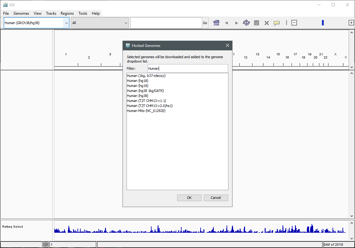
Download hg19 reference genome

To add a new genome in IGV go to Genomes > Select Hosted Genome... and then look for the desired Genome. Press OK to download it.

Load a Genome and some Data Tracks - Part I

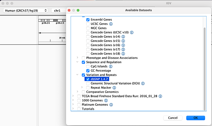
By default, IGV loads the Human GRCh38/hg38 reference genome. If you work with another version of the human genome, or another organism, you can change the genome by clicking the drop down menu in the upper-left corner. For this tutorial, we will be using Human GRCh37/hg19. We will also load additional tracks from the Server using (File -> Load from Server...):

Available Datasets -> Annotations -> Genes > Ensembl Genes
Available Datasets -> Annotations -> Sequence and Regulation -> GC Percentage
Available Datasets -> Annotations -> Variantion and Repeats -> dbSNP 1.4.7
Available Datasets -> Annotations -> Variantion and Repeats -> Repeat Masker

Load a Genome and some Data Tracks - Part II

Load hg19 genome and additional data tracks

Navigation

You should see listing of chromosomes in this reference genome. Choose 1, for chromosome 1.

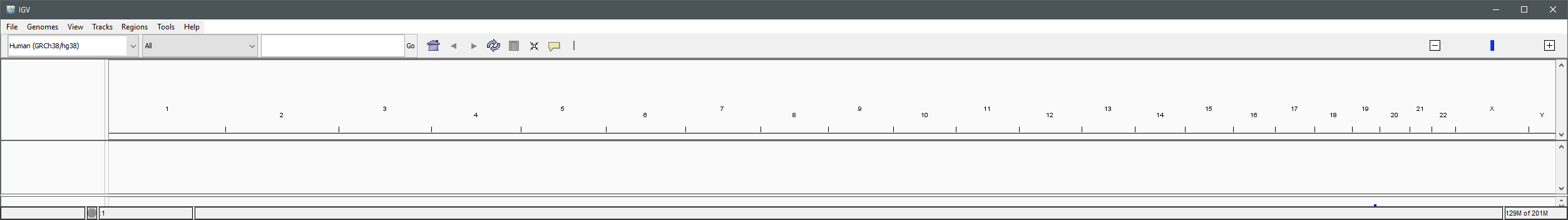
Chromosome chooser

Navigate to chr1:10,000-11,000 by entering this into the location field (in the top-left corner of the interface) and clicking Go. This shows a window of chromosome 1 that is 1,000 base pairs wide and beginning at position 10,000. You can navigate to a gene of interest by typing it in the same box the genomic coordinates are in and pressing Enter/Return. Try it for your favourite gene, or BRCA1 if you can not decide.

Gene model

Genes are represented as lines and boxes. Lines represent intronic regions, and boxes represent exonic regions. The arrows indicate the direction/strand of transcription for the gene. When an exon box become narrower in height, this indicates a UTR.

Gene

When loaded, tracks are stacked on top of each other. You can identify which track is which by consulting the label to the left of each track.

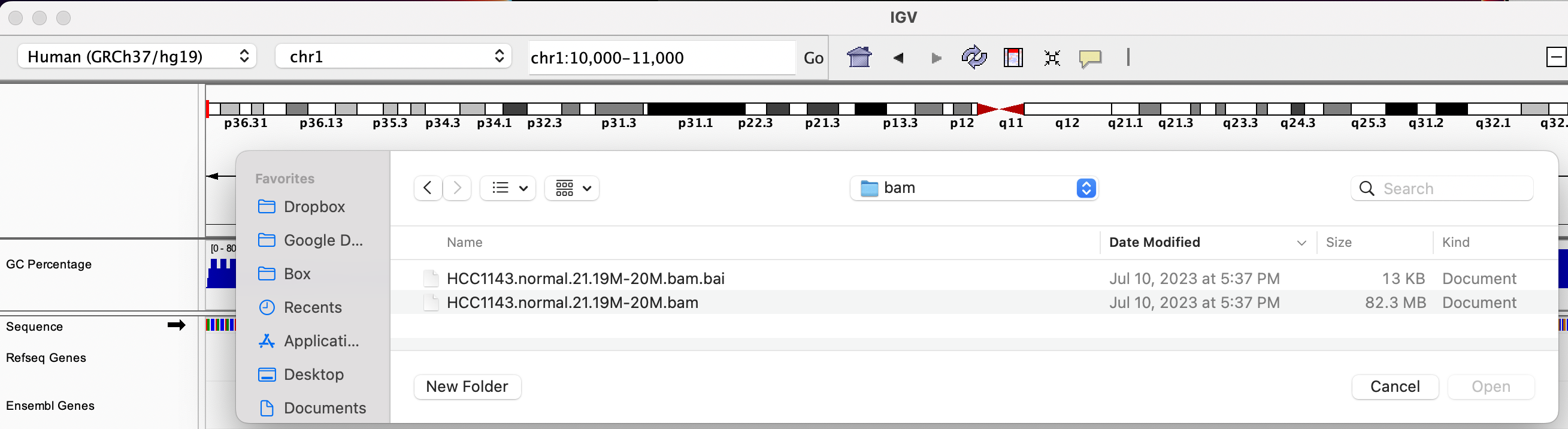
Loading Read Alignments

We will be using the breast cancer cell line HCC1143 to visualize alignments. For speed, only a small portion of chr21 will be loaded (19M:20M). Dowanload HCC1143.normal.21.19M-20M.bam and HCC1143.normal.21.19M-20M.bam.bai from the Git repository to your local drive. In IGV select Human (GRCh37/hg19) reference genome. Then choose File > Load from File..., select the bam file, and click OK. Note that the bam and index files must be in the same directory for IGV to load these properly.

HCC1143 Alignments to hg19

Visualizing read alignments - Part I

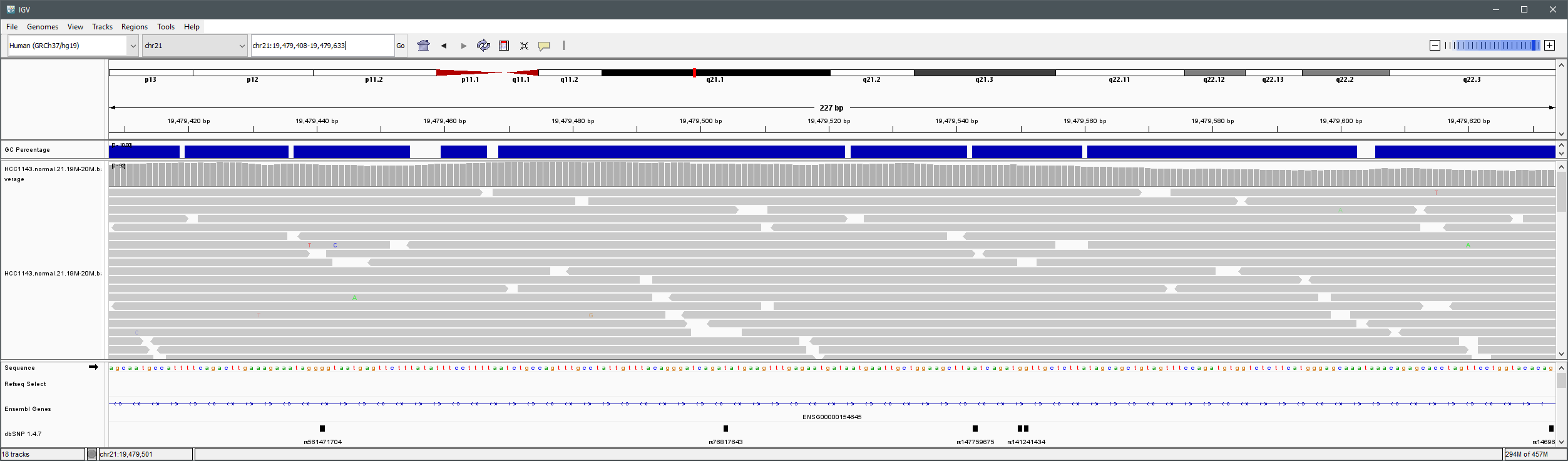
Navigate to a narrow window on chromosome 21: chr21:19,480,041-19,480,386.

To start our exploration, right-click on the read alignment track, and select the following options:

Sort alignments by -> start location
Group alignments by -> pair orientation

Visualizing read alignments - Part II

Experiment with the various settings by right clicking the read alignment track and toggling the options. Think about which would be best for specific tasks (e.g. quality control, SNP calling, CNV finding).

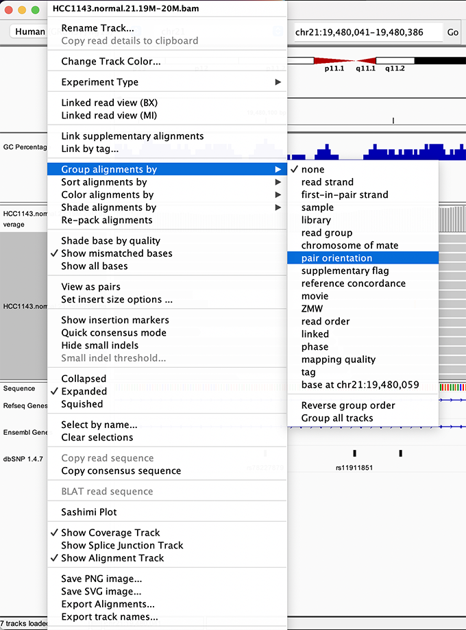
Changing how read alignments are sorted, grouped, and colored

Visualizing read alignments - Part III

You will see reads represented by grey or white bars stacked on top of each other, where they were aligned to the reference genome. The reads are pointed to indicate their orientation (i.e. the strand on which they are mapped).

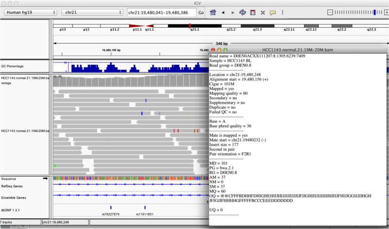
Mouse over any read and notice that a lot of information is available. To toggle read display from hover to click, select the yellow box and change the setting.

Viewing read information for a single aligned read

Inspecting SNPs, SNVs, and SVs

In this section we will be looking in detail at 8 positions in the genome, and determining whether they represent real events or artifacts.

Two neighbouring SNPs

Navigate to region chr21:19,479,237-19,479,814
Note two heterozygous variants, one corresponds to a known dbSNP (G/T on the right) the other does not (C/T on the left)
Zoom in and center on the C/T SNV on the left, sort by base (window chr21:19,479,321 is the SNV position)
Sort alignments by base
Color alignments by read strand

Good quality SNVs/SNPs

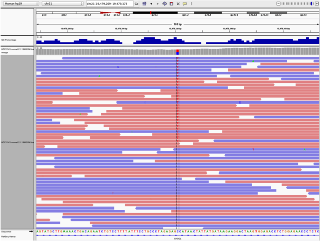
High base qualities in all reads except one (where the alt allele is the last base of the read)
Good mapping quality of reads, no strand bias, allele frequency consistent with heterozygous mutation

Homopolymer region with indel - Part I

Navigate to position chr21:19,518,412-19,518,497

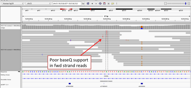
Group alignments by read strand
Center on the A within the homopolymer run (chr21:19,518,470), and Sort alignments by -> base

Homopolymer region with indel - Part II

Center on the one base deletion (chr21:19,518,452), and Sort alignments by -> base

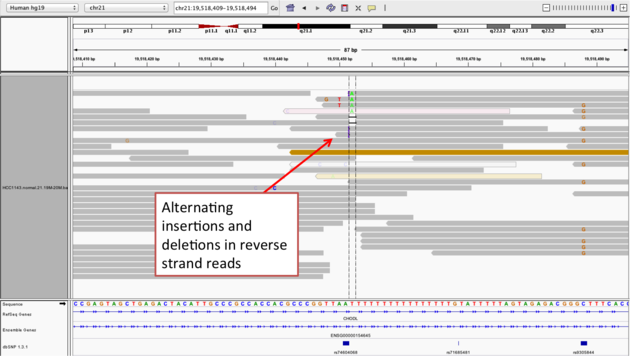
The alt allele is either a deletion or insertion of one or two Ts
The remaining bases are mismatched, because the alignment is now out of sync

Coverage by GC

Navigate to position chr21:19,611,925-19,631,555. Note that the range contains areas where coverage drops to zero in a few places.

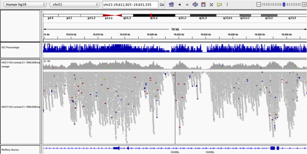
Use Collapsed view
Color alignments by -> insert size and pair orientation
Group alignments by -> none.
Load GC track (if not already loaded above)
See concordance of coverage with GC conten

Heterozygous SNPs

Navigate to region chr21:19,666,833-19,667,007 Sort by base (at position chr21:19,666,901)

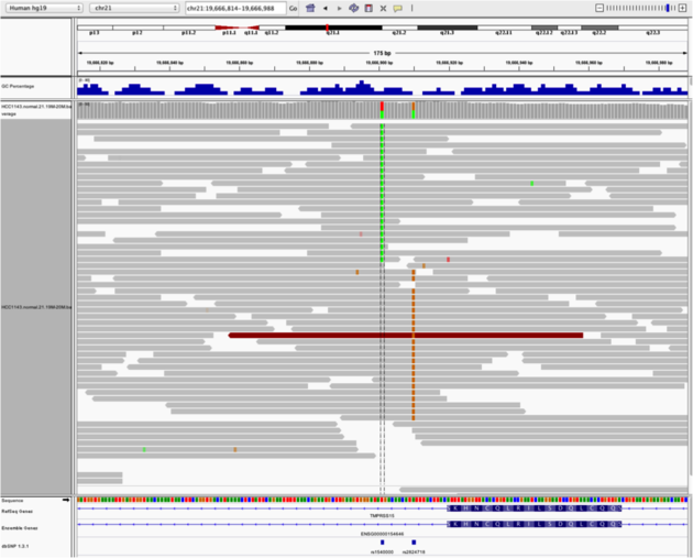
There is no linkage between alleles for these two SNPs because reads covering both only contain one or the other

Low mapping quality

Navigate to region chr21:19,800,320-19,818,162

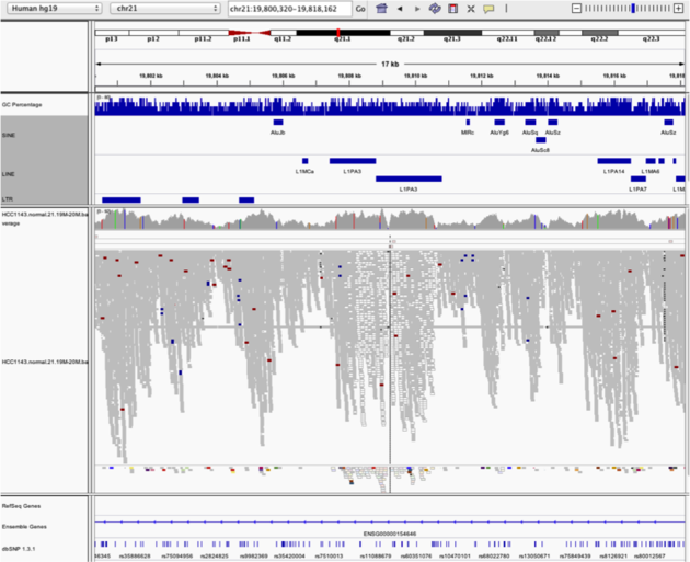
Mapping quality plunges in all reads (white instead of grey). Once we load repeat elements, we see that there are two LINE elements that cause this.

Homozygous deletion - Part I

Navigate to region chr21:19,324,469-19,331,468

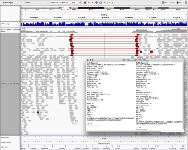
Homozygous deletion - Part II

Then

Turn on View as Pairs and Expanded view
Use Color alignments by -> insert size and pair orientation
Sort reads by insert size
Click on a red read pair to pull up information on alignments

Note:

Typical insert size of read pair in the vicinity: 350bp
Insert size of red read pairs: 2,875bp
This corresponds to a homozygous deletion of 2.5kb

Mis-alignment - Part I

Navigate to region chr21:19,102,154-19,103,108

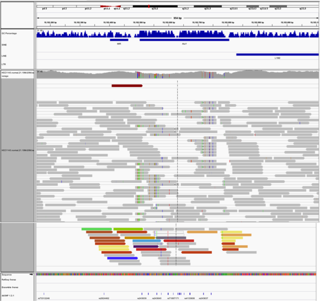
Mis-alignment - Part II

This is a position where AluY element causes mis-alignment.
Misaligned reads have mismatches to the reference and well-aligned reads have partners on other chromosomes where additional AluY elements are encoded.
Zoom out until you can clearly see the contrast between the difficult alignment region (corresponding to an AluY) and regions with clean alignments on either side

Translocation

Navigate to region chr21:19,089,694-19,095,362

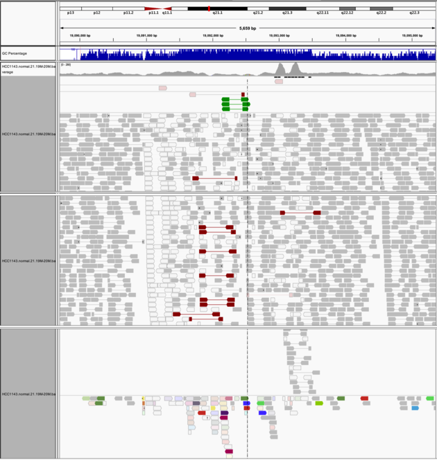
Expanded view
Color alignments by -> insert size and pair orientation
Many reads with mismatches to reference
Read pairs in RL pattern (instead of LR pattern)
Region is flanked by reads with poor mapping quality (white instead of grey)
Presence of reads with pairs on other chromosomes (coloured reads at the bottom when scrolling down)

End of IGV tutorial

3. Data Quality

The First Step to Confident Calls

Quality Control of BAM Files – Part I

We will begin our exercises using pre-aligned BAM files. Start by downloading the dataset from the provided source. The directory structure is as follows:

alignments: contains BAM files for tumor and normal samples.
reference: contains the genome FASTA file and target intervals.
resources: includes variant files (VCF) from resources such as the 1000 genomes project and gnomAD, and subsets of the clinvar and alphamissense databases.
scripts: an empty folder for storing your scripts.

Quality control of the bam files – Part II

The dataset was prepared by the developers of the Precision medicine bioinformatics course at the Griffith lab (McDonnell Genome Institute, Washington University).

It consists of whole-exome sequencing data from cell lines derived from:

A triple-negative breast cancer tumor HCC1395
Matched normal tissue HCC1395 BL

Quality control of the bam files – Part III

We begin by examining the BAM file headers to understand file content and processing details (samtools view -H). Use the following command to inspect the headers:


							samtools view -H ../alignments/normal.recal.bam

Quality control of the bam files – Part IV

The output should include header lines containing information about the BAM file structure and processing.


							@HD     VN:1.6  SO:coordinate
							@SQ     SN:chr6 LN:170805979
							@SQ     SN:chr17        LN:83257441
							@RG     ID:HWI-ST466.C1TD1ACXX.normal   LB:normal       PL:ILLUMINA     SM:normal       PU:HWI-ST466.C1TD1ACXX
							@PG     ID:bwa  PN:bwa  VN:0.7.17-r1188 CL:bwa mem /config/data/reference//ref_genome.fa /config/data/reads/normal_R1.fastq.gz /config/data/reads/normal_R2.fastq.gz
							@PG     ID:samtools     PN:samtools     PP:bwa  VN:1.21 CL:samtools sort
							@PG     ID:samtools.1   PN:samtools     PP:samtools     VN:1.21 CL:samtools view -bh
							@PG     ID:MarkDuplicates       VN:Version:4.5.0.0      CL:MarkDuplicates --INPUT /config/data/alignments/normal.rg.bam --OUTPUT /config/data/alignments/normal.rg.md.bam --METRICS_FILE /config/data/alignments/marked_dup_metrics_normal.txt --MAX_SEQUENCES_FOR_DISK_READ_ENDS_MAP 50000 --MAX_FILE_HANDLES_FOR_READ_ENDS_MAP 8000 --SORTING_COLLECTION_SIZE_RATIO 0.25 --TAG_DUPLICATE_SET_MEMBERS false --REMOVE_SEQUENCING_DUPLICATES false --TAGGING_POLICY DontTag --CLEAR_DT true --DUPLEX_UMI false --FLOW_MODE false --FLOW_QUALITY_SUM_STRATEGY false --USE_END_IN_UNPAIRED_READS false --USE_UNPAIRED_CLIPPED_END false --UNPAIRED_END_UNCERTAINTY 0 --FLOW_SKIP_FIRST_N_FLOWS 0 --FLOW_Q_IS_KNOWN_END false --FLOW_EFFECTIVE_QUALITY_THRESHOLD 15 --ADD_PG_TAG_TO_READS true --REMOVE_DUPLICATES false --ASSUME_SORTED false --DUPLICATE_SCORING_STRATEGY SUM_OF_BASE_QUALITIES --PROGRAM_RECORD_ID MarkDuplicates --PROGRAM_GROUP_NAME MarkDuplicates --READ_NAME_REGEX  --OPTICAL_DUPLICATE_PIXEL_DISTANCE 100 --MAX_OPTICAL_DUPLICATE_SET_SIZE 300000 --VERBOSITY INFO --QUIET false --VALIDATION_STRINGENCY STRICT --COMPRESSION_LEVEL 2 --MAX_RECORDS_IN_RAM 500000 --CREATE_INDEX false --CREATE_MD5_FILE false --help false --version false --showHidden false --USE_JDK_DEFLATER false --USE_JDK_INFLATER false PN:MarkDuplicates
							@PG     ID:GATK ApplyBQSR       VN:4.5.0.0      CL:ApplyBQSR --output /config/project/data/alignments/normal.recal.bam --bqsr-recal-file /config/project/data/alignments/normal.bqsr.recal.table --input /config/project/data/alignments/normal.rg.md.bam --preserve-qscores-less-than 6 --use-original-qualities false --quantize-quals 0 --round-down-quantized false --emit-original-quals false --global-qscore-prior -1.0 --interval-set-rule UNION --interval-padding 0 --interval-exclusion-padding 0 --interval-merging-rule ALL --read-validation-stringency SILENT --seconds-between-progress-updates 10.0 --disable-sequence-dictionary-validation false --create-output-bam-index true --create-output-bam-md5 false --create-output-variant-index true --create-output-variant-md5 false --max-variants-per-shard 0 --lenient false --add-output-sam-program-record true --add-output-vcf-command-line true --cloud-prefetch-buffer 40 --cloud-index-prefetch-buffer -1 --disable-bam-index-caching false --sites-only-vcf-output false --help false --version false --showHidden false --verbosity INFO --QUIET false --use-jdk-deflater false --use-jdk-inflater false --gcs-max-retries 20 --gcs-project-for-requester-pays  --disable-tool-default-read-filters false PN:GATK ApplyBQSR
							@PG     ID:samtools.2   PN:samtools     PP:samtools.1   VN:1.18 CL:samtools view -H ../alignments/normal.recal.bam

Quality control of the bam files – Part V

1) BAM file sorting: How is the bam file sorted?

From the @HD tag, we can see that the bam file is sorted by coordinate

2) Reference genome: Which chromosomes were used as reference?

Lines starting with @SQ indicate that chromosomes 6 and 17 were used as the reference genome.

3) Aligner: Which aligner was used?

The @PG tag shows the processing program. Here, the aligner used was bwa mem.

Quality control of the bam files – Part VI

Next, we examine the alignment body. Start by inspecting a few alignment lines (samtools view):

1) What is likely the read length used?

Run samtools view

						
									samtools view ../alignments/normal.recal.bam | head -3
									HWI-ST466:135068617:C1TD1ACXX:7:1114:9733:82689 163     chr6    60001   60      100M    =       60106   205     GATCTTATATAACTGTGAGATTAATCTCAGATAATGACACAAAATATAGTGAAGTTGGTAAGTTATTTAGTAAAGCTCATGAAAATTGTGCCCTCCATTC   ;B@EDB@A@A@DDDGBGBFCBC?DBEEGCGCAADAGCECDCDDDBABAGBECEGCBHH@?EGBCBCDDBHBAEEHGDFBBHBDDDBCHBGEFFEGEDBBG   MC:Z:100M       MD:Z:100        PG:Z:MarkDuplicates     RG:Z:HWI-ST466.C1TD1ACXX.normalNM:i:0  AS:i:100        XS:i:0
									HWI-ST466:135068617:C1TD1ACXX:7:1303:2021:90688 99      chr6    60001   60      100M    =       60104   203     GATCTTATATAACTGTGAGATTAATCTCAGATAATGACACAAAATATAGTGAAGTTGGTAAGTTATTTAGTAAAGCTCATGAAAATTGTGCCCTCCATTC   >A@FDB@A?@>DDCE@FAF@?BAC>ECFCGBAADBEADBDCDDD@@A@FAFADD?ABF@@EF?@ABCDAFB?DCGEBEB@EBCDCBCHBFEFFDGFCBBG   MC:Z:100M       MD:Z:100        PG:Z:MarkDuplicates     RG:Z:HWI-ST466.C1TD1ACXX.normalNM:i:0  AS:i:100        XS:i:0
									HWI-ST466:135068617:C1TD1ACXX:7:2304:7514:30978 113     chr6    60001   60      2S98M   =       61252   1194    TAGATCTTATATAACTGTGAGATTAATCTCAGATAATGACACAAAATATAGTGAAGTTGGTAAGTTATTTAGTAAAGCTCATGAAAATTGTGCCCTCCAT   >DHABFEACBBBCBGCECHEGBEACBDHCGCHCBDBBFAEAGBCCB@BAEECGBEEDBED>@EDDABDDADE@CBDFFBFBCFCCBADBDBDFFFAFF?@   MC:Z:60S40M     MD:Z:98 PG:Z:MarkDuplicates     RG:Z:HWI-ST466.C1TD1ACXX.normal NM:i:0AS:i:98  XS:i:0

From the CIGAR strings ( 100M, 100M, 2S98M ), we infer that the original reads were 100 base pairs in length.

Quality control of the bam files – Part VII

We can also summarize alignment statistics using samtools flagstat.

1) Create a bash script in the scripts folder named 01_samtools_flagstat.sh to summarize the tumor BAM file.

Write into your bash script the following instruction.


								#!/bin/bash
								samtools flagstat ../alignments/tumor.recal.bam

Make the script executable:


								chmod +x 01_samtools_flagstat.sh

Run the script:


								./01_samtools_flagstat.sh

Quality control of the bam files – Part VIII

The output look like this

						
						16674562 + 0 in total (QC-passed reads + QC-failed reads)
						16663310 + 0 primary
						0 + 0 secondary
						11252 + 0 supplementary
						1871521 + 0 duplicates
						1871521 + 0 primary duplicates
						16582919 + 0 mapped (99.45% : N/A)
						16571667 + 0 primary mapped (99.45% : N/A)
						16663310 + 0 paired in sequencing
						8331655 + 0 read1
						8331655 + 0 read2
						16402064 + 0 properly paired (98.43% : N/A)
						16480080 + 0 with itself and mate mapped
						91587 + 0 singletons (0.55% : N/A)
						23890 + 0 with mate mapped to a different chr
						15733 + 0 with mate mapped to a different chr (mapQ>=5)

Quality control of the bam files – Part IX

The output provides basic statistics, including:

Total number of reads
Number of alignments marked as duplicates

2) How many reads are in the bam files? And how many alignments are marked as duplicate?

For the tumor BAM file, there are 16,674,562 reads and 1,871,521 duplicate alignments.

Quality control of the bam files – Part X

The BAM files appear ready for variant analysis:

High read counts and alignment rates
Read groups are present
Duplicates are marked
Files are sorted by coordinate

Since this is whole-exome sequencing (WES) data, we also need to evaluate whether reads align to the target regions and assess coverage. This can be done using gatk gatk CollectHsMetrics.

Create a script 02_gatk_collecthsmetrics.sh to run gatk CollectHsMetrics on both BAM files.

Quality control of the bam files – Part XI

Example output from CollectHsMetrics shows raw coverage and target enrichment statistics.


						#!/bin/bash
						ALIGNDIR=../alignments
						REFDIR=../reference
						RESOURCEDIR=../resources
						for sample in tumor normal
						do
							singularity exec\
							--bind /storage \
							depot.galaxyproject.org-singularity-gatk4-4.4.0.0--py36hdfd78af_0.img \
							gatk CollectHsMetrics \
							-I "$ALIGNDIR"/"$sample".recal.bam \
							-O "$ALIGNDIR"/"$sample".recal.bam_hs_metrics.txt \
							-R "$REFDIR"/ref_genome.fa \
							--BAIT_INTERVALS "$REFDIR"/exome_regions.bed.interval_list \
							--TARGET_INTERVALS "$REFDIR"/exome_regions.bed.interval_list
						done

Quality control of the bam files – Part XII

To simplify interpretation, parse the metrics using Multiqc. Create a script 03_multiqc.sh and run:


						singularity exec --bind /storage multiqc_latest.sif multiqc ../alignments/

This generates a multiqc_report.html file with hybrid-selection metrics. Documentation for these metrics is available here.

Quality control of the bam files – Part XIII

Check the report (multiqc_report.html) generated by Multiqc hybrid-selection metrics.

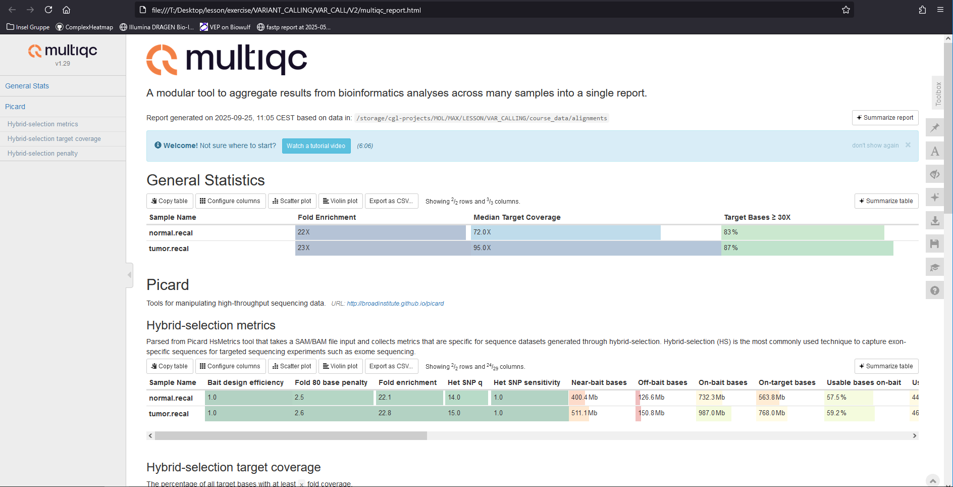
Quality control of the bam files – Part XIV

Key observations from hybrid-selection metrics:

1) Hybrid capture efficiency: How did the hybrid capture go?

Fold enrichment is approximately 22.

2) On-target bases: Are most bases on-target?

About 45% of usable bases are on-target.
Approximately 90% of bases are within 250 bp of target regions (selected bases).

3) Coverage: What kind of coverages can we expect in the target regions?

De-duplicated coverage is 84x for the normal sample and 114x for the tumor sample, indicating sufficient coverage for downstream analysis.

End of Quality Control of BAM files

4. Variant Calling

The Art of Finding Genetic Changes

Variant Calling - Part I

After performing quality control on the BAM files, we can proceed to variant calling. For this tutorial, we will use Mutect2, a somatic variant caller from GATK (Broad Institute).

In addition to the BAM files and the reference genome, Mutect2 requires several important inputs:

--intervals: defines the target regions to analyze, provided in the interval_list format.
-normal: the sample name of the matched normal sample, i.e. the SM tag in the read group header.
--germline-resource: a set of known germline variants with population allele frequencies. This helps estimate the probability that a variant in the normal sample is germline.
--panel-of-normals: a VCF of technical artifact sites derived from normal samples.

Variant Calling - Part II

Create a script called 04_run_mutect2.sh. Consult the Mutect2 manual and replace the FIXME placeholders in the command with the appropriate values for your data.

Then, run the script.


						#!/bin/bash
						
						ALIGNDIR=../alignments
						REFDIR=../reference
						RESOURCEDIR=../resources
						VARIANTDIR=../variants
						
						mkdir -p $VARIANTDIR
						
						singularity exec --bind /storage gatk4.img \
						gatk Mutect2 \
						-R FIXME \
						--intervals "$REFDIR"/exome_regions.bed.interval_list \
						-I FIXME \
						-normal FIXME \
						--germline-resource "$RESOURCEDIR"/af-only-gnomad.hg38.subset.vcf.gz \
						--panel-of-normals "$RESOURCEDIR"/1000g_pon.hg38.subset.vcf.gz \
						-O "$VARIANTDIR"/somatic.vcf.gz

Variant Calling - Part III

💡 Hint:: To obtain the sample name (SM tag) from a BAM file, required for the --normal, you can type:


						singularity exec --bind /storage samtools.sif \
						samtools view -H ../alignments/normal.recal.bam | grep '@RG'

You should get


						@RG     ID:HWI-ST466.C1TD1ACXX.normal   LB:normal       PL:ILLUMINA     SM:normal      PU:HWI-ST466.C1TD1ACXX

Variant Calling - Part IV

Solution


						#!/bin/bash

						ALIGNDIR=../alignments
						REFDIR=../reference
						RESOURCEDIR=../resources
						VARIANTDIR=../variants

						mkdir -p $VARIANTDIR

						singularity exec --bind /storage gatk4.img \
						gatk Mutect2 \
						-R "$REFDIR"/ref_genome.fa \
						--intervals "$REFDIR"/exome_regions.bed.interval_list \
						-I "$ALIGNDIR"/tumor.recal.bam \
						-I "$ALIGNDIR"/normal.recal.bam \
						-normal normal \
						--germline-resource "$RESOURCEDIR"/af-only-gnomad.hg38.subset.vcf.gz \
						--panel-of-normals "$RESOURCEDIR"/1000g_pon.hg38.subset.vcf.gz \
						-O "$VARIANTDIR"/somatic.vcf.gz

Variant Calling - Part V

Once variants have been called, the next step is an initial filtering using FilterMutectCalls.

This step accounts for:

potential technical artifacts,
possible germline variants, and
sequencing errors.

It calculates an error probability and seeks to balance recall (keeping true variants) and precision (removing false positives).

Variant Calling - Part VI

Create a script called 05_filter_mutect_calls.sh and run the filtering command on your Mutect2 output.

						
						#!/bin/bash

						REFDIR=../reference
						VARIANTDIR=../variants

						# fill the filter column
						singularity exec --bind /storage gatk4.img \
						gatk FilterMutectCalls \
						-R "$REFDIR"/ref_genome.fa \
						-V "$VARIANTDIR"/somatic.vcf.gz \
						-O "$VARIANTDIR"/somatic.filtered.vcf.gz

						# create a vcf with variants passing filters (PASS)
						bcftools view -f PASS "$VARIANTDIR"/somatic.filtered.vcf.gz -Oz \
						> "$VARIANTDIR"/somatic.filtered.PASS.vcf.gz

						singularity exec --bind /storage bcftools.img bcftools index --tbi "$VARIANTDIR"/somatic.filtered.PASS.vcf.gz

Questions to consider:

1) How many variants remain after filtering?

	
							zcat ../variants/somatic.filtered.PASS.vcf.gz | grep -v '^#' | wc -l

2) What were the main reasons variants were filtered out?


								singularity exec --bind /storage bcftools.img bcftools view -H ../variants/somatic.filtered.vcf.gz | cut -f 7 | sort | uniq -c | sort -nr

	
								133 PASS
								 48 weak_evidence
								 26 normal_artifact;strand_bias
								 21 panel_of_normals
								 17 normal_artifact
								 13 normal_artifact;slippage;weak_evidence
								 13 clustered_events;normal_artifact;strand_bias
								 12 germline;multiallelic;normal_artifact;panel_of_normals
								 12 base_qual;normal_artifact;strand_bias
								  9 strand_bias;weak_evidence
								  9 normal_artifact;weak_evidence
								  7 slippage;weak_evidence
								  ...

Variant Calling - Part VII

To take a first look at the variant calls, we can display the top lines of the filtered VCF file (excluding the header) using bcftools view -H:


						singularity exec --bind /storage bcftools.img bcftools view -H ../variants/somatic.filtered.vcf.gz | head

you should get


						chr6    106265  .       A       G       .       map_qual;strand_bias;weak_evidence      AS_FilterStatus=weak_evidence,map_qual,strand_bias;AS_SB_TABLE=599,532|0,9;DP=1180;ECNT=1;GERMQ=93;MBQ=33,36;MFRL=254,410;MMQ=27,27;MPOS=8;NALOD=1.67;NLOD=80.04;POPAF=6;TLOD=3.99  GT:AD:AF:DP:F1R2:F2R1:FAD:SB    0/0:284,1:0.00671:285:125,0:149,1:276,1:173,111,0,1 0/1:847,8:0.01:855:381,3:423,5:816,8:426,421,0,8
						chr6    325357  .       G       A       .       PASS    AS_FilterStatus=SITE;AS_SB_TABLE=1335,1391|205,129;DP=3173;ECNT=1;GERMQ=93;MBQ=35,31;MFRL=221,220;MMQ=50,42;MPOS=24;NALOD=2.98;NLOD=280.33;POPAF=6;TLOD=719.91      GT:AD:AF:DP:F1R2:F2R1:FAD:SB    0/0:982,0:0.001054:982:457,0:456,0:932,0:477,505,0,0    0/1:1744,334:0.161:2078:817,141:790,156:1641,324:858,886,205,129
						chr6    325783  .       G       C       .       PASS    AS_FilterStatus=SITE;AS_SB_TABLE=1331,1364|230,295;DP=3313;ECNT=1;GERMQ=93;MBQ=36,35;MFRL=247,206;MMQ=49,43;MPOS=25;NALOD=3.12;NLOD=291.5;POPAF=3.33;TLOD=1292.31   GT:AD:AF:DP:F1R2:F2R1:FAD:SB    0/0:969,0:0.0009626:969:293,0:266,0:1037,0:502,467,0,0  0/1:1726,525:0.224:2251:474,147:432,119:1826,499:829,897,230,295
						chr6    325901  .       G       A       .       PASS    AS_FilterStatus=SITE;AS_SB_TABLE=1300,1302|188,168;DP=3022;ECNT=2;GERMQ=93;MBQ=30,32;MFRL=242,268;MMQ=40,40;MPOS=28;NALOD=-2.178;NLOD=271.54;POPAF=2.18;TLOD=1030.6 GT:AD:AF:DP:F1R2:F2R1:FAD:PGT:PID:PS:SB 0|0:973,5:0.005447:978:428,4:408,0:968,14:0|1:325901_G_A:325901:472,501,4,1     0|1:1629,351:0.183:1980:762,185:628,148:1610,381:0|1:325901_G_A:325901:828,801,184,167
						chr6    325916  .       GTGCTGTATCTGCTGGTGCCTGGAGAGTCATCTGCGCTGGGCTTCTGCGTCCTGGTGTGTGCAA        G       .       PASS    AS_FilterStatus=SITE;AS_SB_TABLE=2790,2616|195,148;DP=5950;ECNT=2;GERMQ=93;MBQ=36,36;MFRL=243,270;MMQ=47,40;MPOS=22;NALOD=-2.148;NLOD=456.31;POPAF=3.83;TLOD=937.7  GT:AD:AF:DP:F1R2:F2R1:FAD:PGT:PID:PS:SB 0|0:1985,7:0.004142:1992:426,6:401,1:1711,16:0|1:325901_G_A:325901:1014,971,4,3     0|1:3421,336:0.116:3757:729,161:631,130:2913,371:0|1:325901_G_A:325901:1776,1645,191,145
						chr6    1742560 .       A       G       .       panel_of_normals        AS_FilterStatus=SITE;AS_SB_TABLE=72,96|31,50;DP=262;ECNT=1;GERMQ=93;MBQ=32,33;MFRL=219,241;MMQ=60,60;MPOS=27;NALOD=1.69;NLOD=14.14;PON;POPAF=0.364;TLOD=235.6       GT:AD:AF:DP:F1R2:F2R1:FAD:SB    0/0:48,0:0.02:48:26,0:17,0:47,0:20,28,0,0       0/1:120,81:0.41:201:44,33:61,42:111,77:52,68,31,50
						chr6    1916336 .       G       A       .       PASS    AS_FilterStatus=SITE;AS_SB_TABLE=68,47|39,26;DP=193;ECNT=1;GERMQ=83;MBQ=30,33;MFRL=233,234;MMQ=60,60;MPOS=26;NALOD=1.65;NLOD=13.24;POPAF=1.44;TLOD=187.23   GT:AD:AF:DP:F1R2:F2R1:FAD:SB    0/0:46,0:0.022:46:12,0:29,0:44,0:31,15,0,0      0/1:69,65:0.482:134:43,30:20,27:64,60:37,32,39,26
						chr6    1930220 .       GA      TT      .       PASS    AS_FilterStatus=SITE;AS_SB_TABLE=40,169|10,33;DP=259;ECNT=1;GERMQ=93;MBQ=37,34;MFRL=229,210;MMQ=60,60;MPOS=21;NALOD=1.79;NLOD=18.36;POPAF=6;TLOD=152.54     GT:AD:AF:DP:F1R2:F2R1:FAD:SB    0/0:64,0:0.016:64:29,0:27,0:61,0:11,53,0,0      0/1:145,43:0.207:188:53,21:83,15:141,36:29,116,10,33
						chr6    2674999 .       A       C       .       PASS    AS_FilterStatus=SITE;AS_SB_TABLE=75,17|50,10;DP=155;ECNT=1;GERMQ=63;MBQ=35,36;MFRL=224,222;MMQ=60,60;MPOS=23;NALOD=1.54;NLOD=10.23;POPAF=2.4;TLOD=190.32    GT:AD:AF:DP:F1R2:F2R1:FAD:SB    0/0:34,0:0.028:34:19,0:15,0:34,0:27,7,0,0       0/1:58,60:0.514:118:25,22:27,33:53,56:48,10,50,10
						chr6    2834013 .       C       G       .       PASS    AS_FilterStatus=SITE;AS_SB_TABLE=42,87|21,52;DP=214;ECNT=1;GERMQ=93;MBQ=38,36;MFRL=217,242;MMQ=60,60;MPOS=25;NALOD=1.68;NLOD=13.85;POPAF=6;TLOD=245.04      GT:AD:AF:DP:F1R2:F2R1:FAD:SB    0/0:53,0:0.02:53:21,0:22,0:46,0:18,35,0,0       0/1:76,73:0.494:149:31,40:38,30:73,71:24,52,21,52

Variant Calling - Part VIII

This shows the main VCF columns for the first few variants:

CHROM,POS → genomic coordinates of the variant
REF,ALT → reference and alternative alleles
QUAL,FILTER → quality score and applied filters
INFO,FORMAT,SAMPLE columns → detailed annotations (e.g. depth, allele frequency, likelihoods)

👉 At this stage, you should notice that both the INFO and FORMAT fields are populated, which we’ll explore in more detail next.

Variant Calling - Part IX

To explore what the FILTER field contains:


						singularity exec --bind /storage bcftools.img bcftools view -h ../variants/somatic.filtered.vcf.gz | grep "^##FILTER"


						##FILTER=<ID=PASS,Description="All filters passed">
						##FILTER=<ID=FAIL,Description="Fail the site if all alleles fail but for different reasons.">
						##FILTER=<ID=base_qual,Description="alt median base quality">
						##FILTER=<ID=clustered_events,Description="Clustered events observed in the tumor">
						##FILTER=<ID=contamination,Description="contamination">
						##FILTER=<ID=duplicate,Description="evidence for alt allele is overrepresented by apparent duplicates">
						##FILTER=<ID=fragment,Description="abs(ref - alt) median fragment length">
						##FILTER=<ID=germline,Description="Evidence indicates this site is germline, not somatic">
						##FILTER=<ID=haplotype,Description="Variant near filtered variant on same haplotype.">
						##FILTER=<ID=low_allele_frac,Description="Allele fraction is below specified threshold">
						##FILTER=<ID=map_qual,Description="ref - alt median mapping quality">
						##FILTER=<ID=multiallelic,Description="Site filtered because too many alt alleles pass tumor LOD">
						##FILTER=<ID=n_ratio,Description="Ratio of N to alt exceeds specified ratio">
						##FILTER=<ID=normal_artifact,Description="artifact_in_normal">
						##FILTER=<ID=orientation,Description="orientation bias detected by the orientation bias mixture model">
						##FILTER=<ID=panel_of_normals,Description="Blacklisted site in panel of normals">
						##FILTER=<ID=position,Description="median distance of alt variants from end of reads">
						##FILTER=<ID=possible_numt,Description="Allele depth is below expected coverage of NuMT in autosome">
						##FILTER=<ID=slippage,Description="Site filtered due to contraction of short tandem repeat region">
						##FILTER=<ID=strand_bias,Description="Evidence for alt allele comes from one read direction only">
						##FILTER=<ID=strict_strand,Description="Evidence for alt allele is not represented in both directions">
						##FILTER=<ID=weak_evidence,Description="Mutation does not meet likelihood threshold">

The weak_evidence filter indicates that these variants did not meet the likelihood threshold. In practice, this means the combined error probability — accounting for technical artifacts, possible germline variants, and sequencing noise — was too high.

Other filters in Mutect2 are hard filters, which apply strict cutoffs on individual features (e.g., depth, mapping quality).

Next, let’s explore the VCF in more detail to better understand:

what kinds of variants remain, and
characteristics such as their variant allele frequency (VAF).

Variant Calling - Part X

To summarize specific information from the VCF, you can use bcftools query. For example, for getting the likelihood TLOD of variant and depth DP of each sample, you can do the following (for the first 20 variants):


						singularity exec --bind /storage bcftools.img bcftools query \
						-f '%CHROM\t%POS\t%FILTER\t\t%INFO/TLOD\t[%SAMPLE=%DP;]\n' ../variants/somatic.filtered.vcf.gz | head -20

	
							chr6    106265  map_qual;strand_bias;weak_evidence              3.99    normal=285;tumor=855;
							chr6    325357  PASS            719.91  normal=982;tumor=2078;
							chr6    325783  PASS            1292.31 normal=969;tumor=2251;
							chr6    325901  PASS            1030.6  normal=978;tumor=1980;
							chr6    325916  PASS            937.7   normal=1992;tumor=3757;
							chr6    1742560 panel_of_normals                235.6   normal=48;tumor=201;
							chr6    1916336 PASS            187.23  normal=46;tumor=134;
							chr6    1930220 PASS            152.54  normal=64;tumor=188;
							chr6    2674999 PASS            190.32  normal=34;tumor=118;
							chr6    2834013 PASS            245.04  normal=53;tumor=149;
							chr6    2840548 PASS            274.4   normal=45;tumor=183;
							chr6    3110986 weak_evidence           3.03    normal=61;tumor=219;
							chr6    3723708 PASS            266.67  normal=58;tumor=201;
							chr6    4892169 weak_evidence           4.43    normal=41;tumor=201;
							chr6    5103987 germline;multiallelic;normal_artifact;panel_of_normals          13.57,257.27    normal=44;tumor=149;
							chr6    6250887 PASS            260.99  normal=54;tumor=196;
							chr6    7176847 PASS            107.39  normal=36;tumor=116;
							chr6    7585458 PASS            171.88  normal=72;tumor=249;
							chr6    7833697 PASS            122.24  normal=15;tumor=77;
							chr6    7883281 germline                99.5    normal=17;tumor=60;

Variant Calling - Part XI

Alternatively, extract the variant allele frequency (AF) for each sample, and compare it to the FILTER column. You should observe that when the filter is weak_evidence, the tumor’s VAF is typically low.


							singularity exec --bind /storage bcftools.img bcftools query \
							-f '%CHROM\t%POS\t%FILTER\t\t%INFO/TLOD\t[%SAMPLE=%AF;]\n' ../variants/somatic.filtered.vcf.gz | head -20

		
							chr6    106265  map_qual;strand_bias;weak_evidence              3.99    normal=0.00671;tumor=0.01;
							chr6    325357  PASS            719.91  normal=0.001054;tumor=0.161;
							chr6    325783  PASS            1292.31 normal=0.0009626;tumor=0.224;
							chr6    325901  PASS            1030.6  normal=0.005447;tumor=0.183;
							chr6    325916  PASS            937.7   normal=0.004142;tumor=0.116;
							chr6    1742560 panel_of_normals                235.6   normal=0.02;tumor=0.41;
							chr6    1916336 PASS            187.23  normal=0.022;tumor=0.482;
							chr6    1930220 PASS            152.54  normal=0.016;tumor=0.207;
							chr6    2674999 PASS            190.32  normal=0.028;tumor=0.514;
							chr6    2834013 PASS            245.04  normal=0.02;tumor=0.494;
							chr6    2840548 PASS            274.4   normal=0.021;tumor=0.522;
							chr6    3110986 weak_evidence           3.03    normal=0.017;tumor=0.019;
							chr6    3723708 PASS            266.67  normal=0.017;tumor=0.42;
							chr6    4892169 weak_evidence           4.43    normal=0.024;tumor=0.02;
							chr6    5103987 germline;multiallelic;normal_artifact;panel_of_normals          13.57,257.27    normal=0.037,0.825;tumor=0.077,0.834;
							chr6    6250887 PASS            260.99  normal=0.018;tumor=0.459;
							chr6    7176847 PASS            107.39  normal=0.026;tumor=0.319;
							chr6    7585458 PASS            171.88  normal=0.015;tumor=0.283;
							chr6    7833697 PASS            122.24  normal=0.057;tumor=0.513;
							chr6    7883281 germline                99.5    normal=0.05;tumor=0.476;

End of Variant Calling

Back to the Variant Calling I

5. Variant Annotation and Filtering

Turning Variants into Insights

Variant Annotation and Filtering - Part I

Ensembl VEP (Variant Effect Predictor)

VEP is a versatile and widely used tool for annotating, analyzing, and prioritizing genomic variants. In cancer genomics, it plays a key role in assessing the functional consequences of somatic mutations. With VEP, we can address questions such as:

How damaging is a specific somatic mutation, based on reference databases?
What is the impact of this mutation in the cancer type under study?
Is the mutation already known in this cancer?
Is the mutation associated with sensitivity or resistance to certain chemotherapies?

Variant Annotation and Filtering - Part II

Why do we need VEP?

Modern sequencing technologies detect thousands of somatic mutations, which are rarely examined individually. We need systematic tools to summarize, prioritize, and interpret these variants.

VEP helps to:

Classify SNVs consistently.
Highlight the most biologically or clinically relevant variants.
Focus analyses on mutations most likely to have functional consequences.

Variant Annotation and Filtering - Part III

Transcript selection

VEP reports variant consequences across all overlapping transcripts. This can result in multiple annotations per variant. Several strategies exist to simplify this output:

--pick: Selects one consequence per variant using a predefined severity hierarchy (HIGH > MODERATE > LOW > MODIFIER).
--pick_allele: Selects one consequence per variant allele.
--pick_allele_gene: Selects one consequence per variant allele per gene.
--per_gene: Selects one consequence per gene.
--flag_pick: Flags the chosen consequence but retains all other annotations.

Variant Annotation and Filtering - Part IV

Consequence Priority

VEP ranks consequences by predicted severity, prioritizing variants with the greatest potential impact on gene function.

Image from the Ensembl VEP website.

Variant Annotation and Filtering - Part V

Order of severity Priority

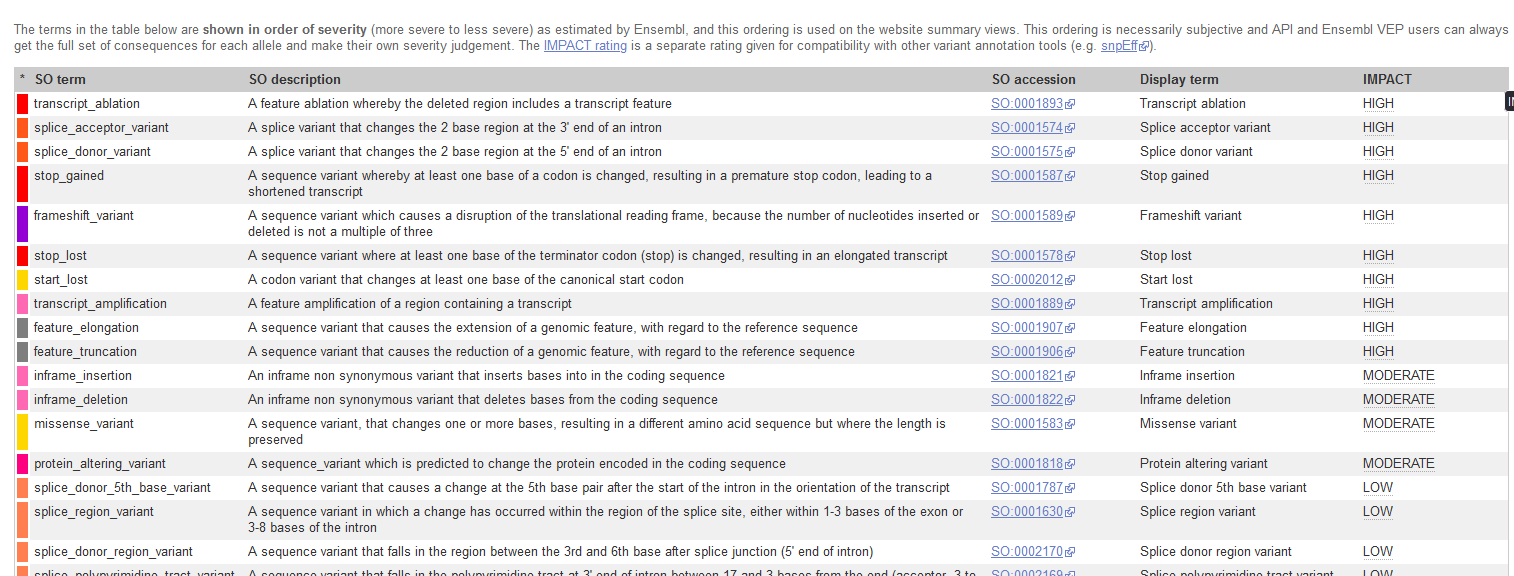
Image from the Ensembl VEP website.

VEP Options and Documentation

To find comprehensive information and all available options for the VEP command-line script:

The Official Source: The Ensembl VEP documentation website provides the definitive guide.
Search for: Ensembl VEP script documentation or VEP command line options.
Key Information to Look For:
- Input/Output formats (VCF, ENSEMBL, etc.)
- Annotation flags ( --sift, --polyphen, --regulatory, --everything)
- Performance options ( --fork, --offline, --cache )
- Custom annotation and Plugin documentation

Consult the documentation before every major run.

Installing the VEP Cache (--dir_cache)

Using a **local cache** is essential for fast and efficient VEP annotation.

What is it? A local copy of all transcript models, regulatory features, and variant data for a species/assembly (e.g., Human GRCh38).
Why use it? Enables offline mode ( --offline ) and provides significantly faster annotation speed compared to connecting to the remote Ensembl database.

How to Install (Recommended):


										# 1. Run the VEP installer script
										perl INSTALL.pl 

										# 2. Select 'y' to install cache files
										# 3. Choose your species and assembly (e.g., homo_sapiens_vep_115_GRCh38)

How to Use in VEP:


									# Use --cache and specify the directory if not using the default ($HOME/.vep)
									./vep -i variants.vcf --cache --dir_cache /path/to/my/cache/

Variant Annotation and Filtering - Part VII

Input data

Copy the following variants into ../variants/cancer_variants.vcf (use tab as column separator)


						##fileformat=VCFv4.2
						#CHROM      POS          ID       REF  ALT  QUAL FILTER  INFO
						chr1     11190510     rs6603781    G    A    .    PASS    .
						chr3    178936091    rs63751289    G    A    .    PASS    .
						chr4     55141055     rs1800744    A    G    .    PASS    .
						chr5    112175770   rs121913343    C    T    .    PASS    .
						chr7     55242465   rs121913529    A    T    .    PASS    .
						chr7    140453136   rs121913530    A    T    .    PASS    .
						chr10    89624230    rs61751507    G    A    .    PASS    .
						chr11   108098576   rs386833395    G    A    .    PASS    .
						chr13    32914438    rs80357090    T    C    .    PASS    .
						chr13    32936646    rs28897743    C    T    .    PASS    .
						chr17     7577121    rs28934578    C    T    .    PASS    .
						chr17     7674894    rs28934574    G    A    .    PASS    .
						chr17    41245466    rs28897686    G    A    .    PASS    .

Variant Annotation and Filtering - Part VIII

Task

Annotate these variants with VEP and identify which genes are affected.

VEP accepts VCF (.vcf or .vcf.gz + index) and several other input formats.

See the VEP input formats documentation

Variant Annotation and Filtering - Part IX

Create a script called 06_vep.sh and run.


							singularity exec --bind /storage vep.sif \
							vep -i cancer_variants.vcf \
								--cache /data/.vep \
								--species homo_sapiens \
								--offline \
								--force_overwrite \
								--assembly GRCh38 \
								--format vcf \
								--symbol \
								--sift b \
								--polyphen b \
								--pick \
								--domains \
								--output_file output.txt

Variant Annotation and Filtering - Part X

Example output


						## VEP command-line: vep --assembly GRCh38 --cache /data/.vep --database 0 --force_overwrite --format vcf --input_file cancer_variants.vcf --offline --output_file output.txt --pick --symbol
						#Uploaded_variation Location    Allele  Gene    Feature Feature_type    Consequence cDNA_position   CDS_position    Protein_position    Amino_acids Codons  Existing_variation  Extra
						rs121913529 chr7:55242465   T   ENSG00000280890 ENST00000626532 Transcript  intron_variant,non_coding_transcript_variant    -   -   -   -   -   -   IMPACT=MODIFIER;STRAND=-1;SYMBOL=ELDR;SYMBOL_SOURCE=HGNC;HGNC_ID=HGNC:49511
						rs28934578  chr17:7577121   T   ENSG00000161960 ENST00000293831 Transcript  missense_variant    597 580 194 D/Y Gac/Tac -   IMPACT=MODERATE;STRAND=1;SYMBOL=EIF4A1;SYMBOL_SOURCE=HGNC;HGNC_ID=HGNC:3282
						rs28897743  chr13:32936646  T   -   -   -   intergenic_variant  -   -   -   -   -   -   IMPACT=MODIFIER
						rs28934574  chr17:7674894   A   ENSG00000141510 ENST00000269305 Transcript  stop_gained 779 637 213 R/* Cga/Tga -   IMPACT=HIGH;STRAND=-1;SYMBOL=TP53;SYMBOL_SOURCE=HGNC;HGNC_ID=HGNC:11998
						rs28897686  chr17:41245466  A   ENSG00000241595 ENST00000334109 Transcript  upstream_gene_variant   -   -   -   -   -   -   IMPACT=MODIFIER;DISTANCE=4221;STRAND=1;SYMBOL=KRTAP9-4;SYMBOL_SOURCE=HGNC;HGNC_ID=HGNC:18902

This example shows rs28934574, a TP53 stop-gained mutation commonly observed in cancer

👉 Try running VEP without --pick or with --everything to explore the difference. Running VEP also produces an output.txt_summary.html file with annotation statistics.

Variant Annotation and Filtering - Part XI

The shortcut option

The shortcut option --everything (-e) expands the annotation with:

--sift b, --polyphen b, --ccds, --hgvs, --symbol, --numbers, --domains,
--regulatory, --canonical, --protein, --biotype, --af, --af_1kg, --af_esp, --af_gnomade, --af_gnomadg, --max_af, --pubmed, --uniprot, --mane, --tsl,
--appris, --variant_class, --gene_phenotype, --mirna

Variant Annotation and Filtering - Part XII

Damage prediction tools

SIFT: Predicts functional impact based on sequence homology and amino acid properties.
PolyPhen: Combines evolutionary, sequence, and structural features for prediction.

Variant Annotation and Filtering - Part XIII

Mutect2 results annotation

In the example above we annotated a simple VCF. Now, let’s extend this to Mutect2 somatic calls from WES of chromosomes 6 and 17.

These calls yield a table of variants, which can be enriched with functional and clinical annotations.

Variant Annotation and Filtering - Part XIV

Extract from the resulting Mutect2 somatic call

Let’s use VEP to annotate this file (use tab as column separator)


							##fileformat=VCFv4.2 
							#CHROM     POS    ID   REF  ALT  QUAL  FILTER  INFO 
							chr6     325357    .    G    A    .     PASS     .
							chr6     325783    .    G    C    .     PASS     .
							chr6     325901    .    G    A    .     PASS     .
							chr6    1916336    .    G    A    .     PASS     .
							chr6    2674999    .    A    C    .     PASS     .
							chr6    2834013    .    C    G    .     PASS     .
							chr6    2840548    .    C    T    .     PASS     .
							chr6    3723708    .    C    G    .     PASS     .
							chr17    745040    .    G    T    .     PASS     .
							chr17   1492466    .    C    T    .     PASS     .
							chr17   2364457    .    T    G    .     PASS     .
							chr17   3433669    .    G    T    .     PASS     .
							chr17   4545725    .    T    C    .     PASS     .
							chr17   4934441    .    G    T    .     PASS     .
							chr17   5007047    .    C    T    .     PASS     .
							chr17   7560755    .    G    A    .     PASS     .
							chr17   7588500    .    G    C    .     PASS     .

Variant Annotation and Filtering - Part XV

The somatic variant call can be annotated with this command


						singularity exec --bind /storage vep.sif \
						vep -i ../resources/Mutect2_data/somatic.filtered.PASS.vcf.gz \
						--cache /data/.vep \
						--species homo_sapiens \
						--assembly GRCh38 \
						--offline \
						--format vcf \
						--symbol \
						--force_overwrite \
						--everything \
						--output_file chr6ch17_mutect2_annotated.txt

Variant Annotation and Filtering - Part XVI

Alternative output formats

VEP can also generate TSV-formatted results.

See the VEP formats documentation.

Variant Annotation and Filtering - Part XVII

interesting variants chr6ch17_mutect2_annotated.txt???

Variant Annotation and Filtering - Part XVIII

Filtering annotated results

When analyzing chr6ch17_mutect2_annotated.txt, we may want to keep only deleterious or moderate/high impact variants.


						singularity exec --bind /storage vep.sif \
						filter_vep \
						-i chr6ch17_mutect2_annotated.txt \
						-o chr6ch17_mutect2_annotated_filtered.txt \
						--filter "(IMPACT is HIGH or IMPACT is MODERATE) or (SIFT match deleterious or PolyPhen match probably_damaging)"

⚠️ Note:

Using OR retrieves variants that meet either criterion.
Using AND is more stringent, keeping only variants supported by both predictions.

Variant Annotation and Filtering - Part XIX

Adding cancer-specific annotations

We can integrate additional resources such as ClinVar for cancer-specific interpretation.

Objective: Add ClinVar data to the VEP output and filter for potentially pathogenic variants

Variant Annotation and Filtering - Part XX

Solution

						
						# Download ClinVar VCF

						# Run VEP with cancer-specific annotations
						singularity exec --bind /storage vep.sif \
						vep -i ../resources/Mutect2_data/somatic.filtered.PASS.vcf.gz \
							--cache /data/.vep \
							--assembly GRCh38 \
							--format vcf \
							--force_overwrite \
							--fork 2 \
							--everything \
							--custom ../resources/clinvar/clinvar.vcf.gz,ClinVar,vcf,exact,0,CLNSIG,CLNREVSTAT,CLNDN \
							--output_file chr6ch17_mutect2_annotated_with_clinVar.txt

						# Filter results
						singularity exec --bind /storage vep.sif \
						filter_vep \
						-i chr6ch17_mutect2_annotated_with_clinVar.txt \
						-o chr6ch17_mutect2_annotated_with_clinVar_filtered.txt \
						--force_overwrite \
						--filter "(IMPACT is HIGH or IMPACT is MODERATE) or \
						(SIFT match deleterious or PolyPhen match probably_damaging) or \
						(ClinVar_CLNSIG match pathogenic)"

						# Generate summary (using simple grep/awk commands)
						echo "Mutation Type Summary:" > summary.txt
						grep -v "#" chr6ch17_mutect2_annotated_with_clinVar_filtered.txt | cut -f7 | sort | uniq -c >> summary.txt

Variant Annotation and Filtering - Part XXI

ClinVar interpretation categories

Pathogenic: Strong evidence variant causes disease
Likely pathogenic: Probable disease-causing
Uncertain significance (VUS): Insufficient evidence
Likely benign: Probably not disease-causing
Benign: Strong evidence variant is harmless
Conflicting: interpretations: Different submitters disagree
Not provided: No interpretation given
Drug response: Affects response to therapy
Other: Miscellaneous interpretations

Variant Annotation and Filtering - Part XXII

Visualization

Once VEP annotations are ready (e.g., chr6ch17_mutect2_annotated_with_clinVar.txt),we can visualize results in R:

Distribution of variant consequences
Consequences by chromosome
Consequences colored by predicted impact
Most common variant classes
Most common biotypes

Variant Annotation and Filtering - Part XXIII

Examples of possible plots in R


							# get libraries
							library(tidyverse);library(magrittr)
							# VEP output in
							vep_data <- read.table("chr6ch17_mutect2_annotated_with_clinVar.txt", 
												   header=F, 
												   sep="\t", 
												   comment.char="#")
							# The standard VEP column names are:
							colNames <- c("#Uploaded_variation", "Location", "Allele", "Gene", "Feature", "Feature_type",
							"Consequence", "cDNA_position", "CDS_position", "Protein_position", "Amino_acids",
							"Codons", "Existing_variation", "Extra")
							# Set column names
							colnames(vep_data) <- colNames
							# Split when it contains multiple values
							consequences_df <- vep_data %>%
							  separate_rows(Consequence, sep="&") %>%
							  select(Consequence)
							# get chr
							vep_data <- vep_data %>%
							  separate(Location, into = c("chr", "position"), sep=":") %>% 
							  mutate(chr = factor(chr, levels = c("chr6", "chr17")))
							# Extract IMPACT from Extra column
							vep_data$IMPACT <- gsub(".*IMPACT=([^;]+).*", "\\1", vep_data$Extra)
							# get nice data out of the df
							extract_field <- function(data, field) {
							  gsub(paste0(".*", field, "=([^;]+).*"), "\\1", data$Extra)
							}
							# combine multiple fields
							  mutate(
								IMPACT = extract_field(., "IMPACT"),
								SYMBOL = extract_field(., "SYMBOL"),
								VARIANT_CLASS = extract_field(., "VARIANT_CLASS"),
								BIOTYPE = extract_field(., "BIOTYPE")
							  )

Variant Annotation and Filtering - Part XXIV

Next steps

With an annotated set of somatic variants, we can:

Add other databases (COSMIC, CancerHotspots, OncoKB, etc.).
Use additional VEP plugins depending on the biological question.
Investigate candidate driver genes.
Consider population frequencies (to exclude common variants).
Assess drug–gene interactions.
Explore the literature for functional insights.
Visualize results for clearer interpretation.

Variant Annotation and Filtering - Part XXV

1. Consequence plot, to visualize the distribution of consequences


						# consequence plot
						ggplot(vep_data, aes(x=reorder(Consequence, table(Consequence)[Consequence]))) +
						  geom_bar() +
						  coord_flip() +
						  theme_minimal() +
						  labs(title="Distribution of \n Variant Consequences",
							   x="Consequence Type",
							   y="Count")

Variant Annotation and Filtering - Part XXVI

2. Consequence plot, by chromosome


						# consequence plot 
						ggplot(vep_data, aes(x=reorder(Consequence, table(Consequence)[Consequence]))) +
						  geom_bar() +
						  coord_flip() +
						  theme_minimal() +
						  labs(title="Distribution of \n Variant Consequences",
							   x="Consequence Type",
							   y="Count") +
						  facet_grid(~chr) +
						  theme(
							legend.position = "bottom"
						  )

Variant Annotation and Filtering - Part XXVII

3. Can we see the consequence colored by impact


						# Impact + Consequence plot
						ggplot(vep_data, aes(x=reorder(Consequence, table(Consequence)[Consequence]), fill=IMPACT)) +
						  geom_bar() +
						  coord_flip() +
						  theme_minimal() +
						  scale_fill_brewer(palette="Set1") +
						  labs(title="Variant Consequences \n by Impact",
							   x="Consequence Type",
							   y="Count") +
						  theme(
							legend.position = "bottom"
						  )

Variant Annotation and Filtering - Part XXVIII

4. Can we see the consequence colored by impact by chromosome


						# Impact + consequence plot x chr
						ggplot(vep_data, aes(x=reorder(Consequence, table(Consequence)[Consequence]), fill=IMPACT)) +
						  geom_bar() +
						  coord_flip() +
						  theme_minimal() +
						  scale_fill_brewer(palette="Set1") +
						  labs(title="Variant Consequences \n by Impact",
							   x="Consequence Type",
							   y="Count") +
						  facet_grid(~chr) +
						  theme(
							legend.position = "bottom"
						  )

Variant Annotation and Filtering - Part XXIX

5. What are the most common variant classes?


						# variant class plot
						vep_data %>%
						  count(VARIANT_CLASS) %>%  # Count the classees
						  arrange(desc(n)) %>%  # Sort in descending ord
						  ggplot(aes(x = reorder(VARIANT_CLASS, n), y = n)) +
						  geom_bar(stat = "identity", fill = "steelblue") +
						  coord_flip() +
						  theme_minimal() +
						  labs(title = "Distribution of \n Variant Classes",
							   x = "Variant Class",
							   y = "Count")

Variant Annotation and Filtering - Part XXX

6. What are the most common biotypes?


						# biotype distribution
						ggplot(vep_data, aes(x=reorder(BIOTYPE, table(BIOTYPE)[BIOTYPE]))) +
						  geom_bar(fill="steelblue") +
						  coord_flip() +
						  theme_minimal() +
						  labs(title="Distribution of \n Biotypes",
							   x="Biotype",
							   y="Count")

Variant Annotation and Filtering - Part XXXI

References

McLaren W, et al. The Ensembl Variant Effect Predictor. Genome Biology (2016)
Eilbeck K, et al. The Sequence Ontology: a tool for the unification of genome annotations. Genome Biology (2005)
Richards S, et al. Standards and guidelines for the interpretation of sequence variants. Genetics in Medicine (2015).
Cancer variant analysis course, SIB.
Precision medicine bioinformatics course, Griffith labMcDonnell Genome Institute - Washington University.

End of Variant Annotation and Filtering

End

Back to the first slide