Exercises

1. Setup

Tools of the trade

Necessary tools (to be installed)

• samtools
• GRCh37 (hg19) reference genome
• R or python or your preferred scripting language
• MutationaPatterns
• ev. Sigprofiler

samtools Installation 🛠️ - Part I

You can install samtools using a package manager on most operating systems, such as apt for Debian/Ubuntu or brew for macOS. Alternatively, you can download the source code and compile it yourself.

Method 1: Using a Package Manager

This is the recommended method for most users as it's the simplest and most reliable way to install samtools and its dependencies.

For Debian/Ubuntu

							sudo apt-get update
							sudo apt-get install samtools
							

For macOS with Homebrew

							brew install samtools
							

samtools Installation 🛠️ - Part II

Method 2: Compiling from Source

This method gives you more control over the installation, which can be useful for more advanced users or on systems without a package manager.

Download the source code:

Get the latest version from the official samtools website.

Unpack the files:

							tar -xf samtools-.tar.bz2
							cd samtools-
							

samtools Installation 🛠️ - Part III

3. Configure and compile:

							./configure
							make
							make install
							

Verification

To confirm that samtools is installed correctly, run the following command in your terminal. It should display the version number and a list of available commands.

							samtools --version
							

Downloading Genome Reference: GRCh37 - Part I

To perform mutational signature analysis, you need to download a reference genome. We will use GRCh37, also known as hg19. The most reliable way to get this file is from a well-established bioinformatics repository like NCBI or the UCSC Genome Browser.

We recommend using a command-line tool like wget or curl to ensure a stable download, which is crucial for large files.

Method 1: Using wget 📥

This command will download the FASTA file directly from the UCSC Genome Browser's public repository.

						wget http://hgdownload.soe.ucsc.edu/goldenPath/hg19/bigZips/hg19.2bit
						

After downloading, you will need to convert the file to the FASTA format, which is required by samtools.

						wget http://hgdownload.soe.ucsc.edu/goldenPath/hg19/bigZips/hg19.fa.gz
						gunzip hg19.fa.gz
						

Downloading Genome Reference: GRCh37 - Part II

Method 2: Using NCBI's FTP Server 🌐

You can also download the reference from NCBI's FTP server. The command below downloads the gzipped file for GRCh37.p13 and unzips it.

						wget ftp://ftp.ncbi.nlm.nih.gov/genomes/all/GCA/000/001/405/GCA_000001405.14_GRCh37.p13/GCA_000001405.14_GRCh37.p13_genomic.fna.gz
						gunzip GCA_000001405.14_GRCh37.p13_genomic.fna.gz
						

Once you have the FASTA file (.fa or .fna), you must index it to use it with samtools. This process creates a .fai file for fast random access.

						samtools faidx your_genome_file.fa
						

Installing R and Python 🐍 - Part I

This slide will guide you through the process of installing both R and Python, two essential programming languages for data analysis and bioinformatics.

Installing Python

Python is widely used for scripting and data science. The easiest way to get started is by downloading the official installer from the Python website.

1. Download Python: Go to the official Python website and download the latest stable version of Python 3.
2. Run the Installer:
   • Windows: Run the .exe installer. Make sure you check the box that says Add Python to PATH before you click "Install Now." This is a crucial step that allows you to run Python from any command prompt.
   • macOS: Run the .pkg installer. The installer will automatically configure the correct paths for you.
3. Verify Installation: Open your terminal or command prompt and type python --version (or python3 --version on some systems) to confirm the installation.

Installing R and Python 🐍 - Part II

Installing R R is a programming language and environment specifically designed for statistical computing and graphics. We recommend installing it alongside RStudio, a user-friendly Integrated Development Environment (IDE) that makes working with R much easier.

1. Download and Install R: Go to the CRAN website and download the latest version for your operating system.
2. Download and Install RStudio: Go to the RStudio Desktop website and download the free desktop version.
3. Launch RStudio: Open RStudio. You'll see the console where you can start writing R commands.
4. Verify Installation: In the RStudio console, type R.version to display the version information.

Guide to Installing MutationaPatterns 📊 - Part I

MutationaPatterns is a popular Bioconductor R package used for mutational signature analysis. To use it, you'll need to install R and then the MutationaPatterns package from within the R environment.

Step 1: Install R and RStudio First, you need to install R, the programming language, and RStudio, which is a user-friendly interface for R.

1. Download and Install R: Go to the CRAN website and download the latest version for your operating system.
2. Download and Install RStudio: Go to the RStudio website and download the free desktop version.

Guide to Installing MutationaPatterns 📊 - Part II

Step 2: Install BiocManager

MutationaPatterns is part of the BiocManager project, which requires its own package manager, BiocManager. Open RStudio and run the following command in the console to install it.

						install.packages("BiocManager")
						

Guide to Installing MutationaPatterns 📊 - Part III

Step 3: Install MutationaPatterns

Now that BiocManager is installed, you can use it to install MutationaPatterns and all its dependencies.

						BiocManager::install("MutationaPatterns")
						

This command will download and install the package and any other required packages. It may take a few minutes.

Guide to Installing MutationaPatterns 📊 - Part IV

Step 4: Verify the Installation

To check that the installation was successful, load the library and view its version. If no error messages appear, you're ready to start using MutationaPatterns.

						library(MutationaPatterns)
						packageVersion("MutationaPatterns")
						

Installing Sigprofiler 🐍 - Part I

Sigprofiler is a powerful suite of tools for mutational signature analysis, with the main tool being SigProfilerExtractor. It's a Python-based tool, and the easiest way to install it is using the pip package manager.

Step 1: Install Python

First, ensure you have Python 3.8 or newer installed on your system. If not, you can download it from the official Python website.

Step 2: Install SigProfilerExtractor via pip

Open your terminal or command prompt and run the following command to install the main package. This will also install all its dependencies.

						pip install SigProfilerExtractor
						

Installing Sigprofiler 🐍 - Part II

Step 3: Install a Reference Genome 🧬

After installing the main package, you must install at least one reference genome that you'll use for your analysis. This is a separate step that uses a function within the SigProfilerMatrixGenerator module. Open a Python interpreter and run the following commands. Here, we install the GRCh37 (human hg19) reference genome. You can install others as needed.

						from SigProfilerMatrixGenerator import install as genInstall
						genInstall.install('GRCh37')
						

Installing Sigprofiler 🐍 - Part III

Step 4: Verify the Installation

To check if everything is working correctly, you can try importing the main module in your Python interpreter. If no errors appear, the installation was successful.

						from SigProfilerExtractor import sigpro as sig
						

End

2. Mutational Signatures

Deconvolution of mutational processes in cancer genomes.

Exploring VCF Files

The Variant Call Format (VCF) is a standard text file format for storing gene sequence variations. A VCF file is composed of two main parts:

1. Header Lines: Starting with a ##, these lines provide metadata about the file, including:

   • How the body is organized.
   • The types and values to expect in the ID, FILTER, INFO, and FORMAT fields.

2. The Body: This is a tab-separated table that contains the variant information. The last line of the header, which begins with a single #, serves as the column header for this table.

The table typically includes columns like CHROM, POS, ID, REF, ALT, QUAL, FILTER, INFO, FORMAT, and one or more sample names. The values in the sample columns follow the formatting specified by the FORMAT field.

VCF file

Here an example of the first lines of a VCF file:

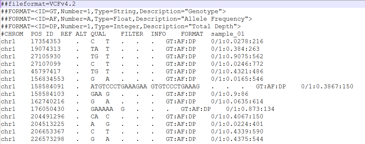
VCF file

Plotting the 6 Mutational Channels

Write a script in R, Python, or your preferred programming language that reads your VCF file and generates a bar plot of the mutation distribution.

Guidelines for the Script:
1. Filtering: Your script should only consider single-nucleotide variants (SNVs). Any mutation where the reference (REF) or alternative (ALT) allele is more than one character should be ignored.
2. Standardization: To simplify analysis, all mutations must be converted to one of the six possible pyrimidine-to-pyrimidine/purine substitutions.
3. Forward Strand Conversion: To ensure consistency, all mutations are converted to the forward strand. For example, G>T mutations (on the reverse strand) are converted to C>A by complementing both nucleotides. This conversion applies to all six possible mutation types: C>A, C>G, C>T, T>A, T>C, T>G.

The final output will be a histogram representing the frequency of each of the six mutational channels.

6 Mutational Channels Plot

You should get something like this

6 mutational channels plot

Code highlights

Here you can find help if you need it for any reason. It is a Python script, so adapt it to your specific case.

Extending to 96 Mutational Channels

To extend your analysis from 6 to 96 channels, you need to incorporate the context of each mutation. This context is determined by the nucleotide immediately before (5') and after (3') the mutation. This results in 96 possible combinations (4 bases for the 5' position, 4 bases for the 3' position, and the 6 mutational types).

Accessing Context with samtools

You can use samtools faidx from the command line to efficiently query the reference genome and retrieve these contextual nucleotides.

						samtools faidx reference.fasta chr:start-end
						

This command returns the sequence of characters from the specified chromosome and genomic coordinates (e.g., chrXXX:aa-bb). You can use this to retrieve the necessary 5' and 3' context for each mutation in your VCF file.

Generating a samtools Script

You will now create a script that automates the process of querying the reference genome using samtools faidx for each mutation in your VCF file. This is an efficient way to retrieve the contextual nucleotides required to expand from 6 to 96 channels.

The Script's Task

Your script (written in R, Python, or a similar language) will read your VCF file line-by-line and generate a series of samtools commands. The generated commands will look like this:

						samtools faidx <reference_genome> <chromosome>:<position>-<position>
						

Running the Script

Once your script has generated the list of samtools commands, you can execute it from your terminal.

1. Make the script executable:

							chmod +x your_script_name.sh
							

2. Run the script:

							./your_script_name.sh
							

This process allows you to automate the retrieval of all necessary contextual information from the reference genome without manually typing out each command.

Samtools index output file

After running samtools index, you obtained a file with two lines for each position, like this:

						>chr1:17354352-17354354
						GCT
						>chr1:27107098-27107100
						GCG
						>chr1:156834552-156834554
						CGC
						>chr1:162740215-162740217
						CGC
						...
						

Preparing the 96-Nucleotide Histogram File

You will now process your data to prepare a file for the 96-nucleotide histogram. This involves combining the mutation information from your VCF file with the contextual data you retrieved using samtools.

The Task:

1. Write a script that reads two lines at a time: one from your original VCF file and the corresponding contextual sequence from the samtools output.
2. For each mutation, determine the trinucleotide context by combining the 5' and 3' nucleotides with the reference base.
3. Generate a new file that lists the following for each mutation:
   • REF (Reference allele)
   • ALT (Alternative allele)
   • TRINUC (The trinucleotide context)

The resulting output file should be a clean, organized table that resembles the example below:

Plotting the 96-Nucleotide Histogram

Using the file you just created, you will now generate a 96-channel bar plot. This type of plot is a fundamental tool in mutational signature analysis, as it provides a comprehensive visualization of all possible single-base substitutions within their trinucleotide context.

The Task:

Write a script in R, Python, or another language of your choice that performs the following steps:

1. Read the file: Your script should read the file containing the REF, ALT, and TRINUC information.
2. Count the substitutions: Count the frequency of each of the 96 possible mutational combinations.
3. Generate the plot: Create a bar plot that visualizes the frequency of each of the 96 combinations. The x-axis should represent the trinucleotide substitutions, and the y-axis should represent their counts or frequencies.

Plot 96 channels

You should obtain something like this

Plot 96 channels

Code highlights

Here you can find help if you need it for any reason. It is a Python script, so adapt it to your specific case.

Preparing Mutational Signatures - Part I

The next step is to prepare your data for mutational signature analysis. This process involves formatting the mutation counts into a matrix that can be used by specialized bioinformatics tools like MutationaPatterns or Sigprofiler.

Your task is to write a script (in R, Python, or a similar language) that:

1. Generates an input file for MutationaPatterns: The script should process your data and write it to a new file in the specific format required by the MutationaPatterns tool. This usually involves creating a table where rows represent the 96 mutational channels and columns represent your samples.

2. Alternatively, use Sigprofiler: If you choose to use Sigprofiler, you can skip this data preparation step, as it is designed to accept your input VCF file directly.

This step is crucial for transitioning from a raw histogram to a format that can be analyzed to identify and extract known or novel mutational signatures.

Code highlights

Here you can find help if you need it for any reason. It is a Python script, so adapt it to your specific case.

Preparing Mutational Signatures - Part II

The next step is to prepare your data for mutational signature analysis. This process involves formatting the mutation counts into a matrix that can be used by specialized bioinformatics tools.

The Task:

Your task is to write a script in R, Python, or a similar language that prepares the input file for your chosen tool. You have two primary options:

1. MutationPatterns: To use this tool, your script must generate a data file in its specific input format. This typically requires creating a matrix where rows correspond to the 96 trinucleotide substitution types and columns represent your samples.

2. Sigprofiler: If you decide to use this tool, you can skip the data preparation step, as Sigprofiler is designed to process the input VCF file directly.

Mutational Signatures: Interpreting Your Results - Part I

You've now successfully completed the computational part of your analysis. The final step is to interpret the results you have achieved, which are the mutational signatures of your sample. These signatures are a combination of a mutational profile (a bar plot) and an exposure value. The exposure represents the number of mutations that are likely caused by a specific mutational signature.

What to Look For:

• Signature Profiles: Your results will include a profile for each identified signature. The profiles are 96-channel bar plots that represent the unique pattern of mutations associated with a specific mutagenic process (e.g., UV exposure, tobacco smoke). By comparing these profiles to known signatures (like those in the COSMIC database), you can infer the aetiology of the mutations.

Mutational Signatures: Interpreting Your Results - Part II

What to Look For:

• Exposure Values: The exposure values are the most important part of your results. They tell you the contribution of each signature to the total mutational burden in your sample. A high exposure value for a signature means that the corresponding mutagenic process had a significant impact on your sample.
• Residual Mutations: Pay attention to any residual mutations that were not assigned to a signature. These unassigned mutations may indicate the presence of a novel or uncharacterized mutational process.

Decomposing Signatures with COSMIC - Part I

You will now use a specialized bioinformatics tool to deconvolve or decompose the mutational signatures you found. This process involves comparing your sample's unique mutational profile to the COSMIC database, which contains a comprehensive list of known mutational signatures and their associated aetiologies (causes).

The Goal:

The objective is to determine which of the known signatures contribute to the overall mutational pattern observed in your data. The result is an exposure value for each COSMIC signature, representing its contribution to your sample's mutational load.

Decomposing Signatures with COSMIC - Part II

Key Steps:

1. Input Your Data: Use the signature file you prepared in the previous step as input for your analysis tool.
2. Compare to COSMIC: The tool will mathematically compare your sample's 96-channel profile to the signatures in the COSMIC database.
3. Decompose the Profile: The tool will break down your sample's profile into a linear combination of the most likely COSMIC signatures.
4. Obtain Exposures: You will receive a list of COSMIC signatures and their corresponding exposure values, indicating their contribution to your sample's mutations.

Analyzing Results and Overfitting - Part I

After comparing your data to the COSMIC signatures, you need to interpret the results with a critical eye. It's not enough to simply see which signatures were found; you must also consider whether the model might have overfitted the data. Overfitting occurs when a model fits the noise or random fluctuations in the data rather than the underlying biological signal. This can lead to a false identification of a signature.

Key Indicators of Overfitting

• High Number of Signatures: If the model identifies an unusually large number of signatures for a single sample, it might be overfitting. A complex model can fit every tiny variation, including noise, by attributing them to a new signature.
• Low Exposure Values: Pay close attention to signatures with very low exposure values. An exposure value close to zero suggests the signature contributed very little to the mutational profile. In these cases, it's possible the model assigned a signature just to account for a few random mutations.

Analyzing Results and Overfitting - Part II

Key Indicators of Overfitting

• High Reconstruction Error: Most mutational signature analysis tools provide a measure of reconstruction error. A high reconstruction error indicates that the model did not accurately replicate the original mutational profile, suggesting a poor fit.
• Biological Plausibility: Consider the biological context. For example, if your sample is from a lung cancer patient who has never smoked, but the model attributes a high exposure to Signature 4 (tobacco smoke), this could be a sign of overfitting.

By checking for these issues, you can ensure that your interpretation of the mutational signatures is robust and biologically meaningful.

End